Even though I have a degree in physics I never learned general relativity properly. I took a differential geometry class and while it was one of my favorite classes at uni, it didn't go beyond 19th century math: curves and surfaces in Euclidean space and things like the Gauss-Bonnet theorem.
One day, YouTube recommended a video from the WE-Heraeus International Winter School on Gravity and Light channel. This channel contains a series of lectures that offer an introduction to the central concepts in general relativity and cosmology. The lectures are really good. They're also quite dense. I've been writing notes while watching them but I also feel the need to write them somewhere more "permanent" so I can easily refer back to them when I inevitably forget a concept later on, and also so I can add to them if something's unclear, etc. Besides, just writing things down again will help fix the concepts in my memory better.
After starting this I found a set of notes by Richie Dadhley which are much polished than anything I could ever write, so you probably want to read those instead. These notes are mainly meant for myself; writing them down helps me retain the concepts in memory and also makes it easier to refresh my memory when I get back to them.
Topological spaces
Spacetime is (roughly) a set. But in physics, we want to talk about continuous maps, and for that you need more structure than bare sets can provide.
The weakest structure on a set that allows for a definition of continuity is a topology.
Definition. Let $M$ be a set and $\mathcal{O}_M$ be a collection of subsets of $M$. We say that $\mathcal{O}_M$ is a topology over $M$ if
The empty set and $M$ are in $\mathcal{O}_M$,
if $U,V$ are in $\mathcal{O}_M$, then $U \cap V$ is in $\mathcal{O}_M$,
if $\{U_i\}_{i \in \mathcal{I}}$ is a collection of sets in $\mathcal{O}_M$ for an arbitrary index set $\mathcal{I}$, then $\bigcup_{i \in \mathcal{I}} U_i$ is in $\mathcal{O}_M$.
So essentially, a topology needs to be closed over finite intersections and arbitrary unions. Some trivial, uninteresting examples of topologies: for any set $M$, $\mathcal{O}_M = \{\emptyset, M\}$ is a topology (known as the chaotic topology) and so is $\mathcal{O}_M = \mathbb{P}(M)$ (the discrete topology). Note that $\{M\}$ does not define a topology over $M$ because we need to include the empty set.
Definition. If $M$ is a set and $\mathcal{O}_M$ is a topology over $M$, then the tuple $(M, \mathcal{O}_M)$ is called a topological space.
Claim. Let $M = \mathbb{R}^d$ and
$$B_r(p) = \{(q_1, \dots, q_d) \in \mathbb{R}^d \mid \sum_i (q_i - p_i)^2 < r\}$$
where $r \in \mathbb{R}^+, p \in \mathbb{R}^d$. Let
$$\mathcal{O}_\mathrm{standard} = \{\mathcal{U} \in \mathbb{P}(M) \mid \forall p \in \mathcal{U} : \exists r \in \mathbb{R}^+ : B_r(p) \subseteq \mathcal{U}\}.$$
Then $\mathcal{O}_\mathrm{standard}$ is a topology over $M = \mathbb{R}^d$, called the standard topology on $\mathbb{R}^d$.
Proof. Let's check the three conditions:
$\emptyset \in \mathcal{O}_s$ vacuously; $\mathbb{R}^d \in \mathcal{O}_s$ because $B_r(p) \subseteq \mathbb{R}^d$ for any $r \in \mathbb{R}^+, p \in \mathbb{R^d}$.
If $V, W \in \mathcal{O}_s$, then let $p \in V \cap W$. This means there are two balls around $p$, one of which is in $V$ and the other in $W$. Pick the smaller of the two: that one is in $V \cap W$. Hence $V \cap W \in \mathcal{O}_s$.
Let $p_i \in \bigcup_{i \in \mathcal{I}} U_i$, so $p_i \in U_i$ for some $i \in \mathcal{I}$. So there's a ball $B_{r_i}(p_i) \in U_i$ for some $r_i > 0$. Clearly $B_{r_i}(p_i) \in \bigcup_{i \in \mathcal{I}} U_i$.
Some terminology: sets in the topology are called open sets, and sets whose complement in $M$ are in the topology are called closed sets. Closed is not the opposite of open: a set can be both open and closed, and can also be neither open nor closed.
Continuous maps
Definition. Let $(M, \mathcal{O}_M), (N, \mathcal{O}_N)$ be topological spaces. Then the function
$$\begin{align*}
f \colon M &\to N \\
m &\mapsto f(m)
\end{align*}$$
is continuous if for every $V \in \mathcal{O}_N$, we have that $f^{-1}(V) \in \mathcal{O}_M$, where $f^{-1}$ is defined as the preimage of $f$: $f^{-1}(V) = \{m \in M \mid f(m) \in V\}$.
Example. $M = N = \{1, 2\}$, $\mathcal{O}_M = \{\emptyset, \{1\}, \{2\}, \{1,2\}\}, \mathcal{O}_N = \{\emptyset, \{1,2\}\}$. Consider the following functions:
$f \colon M \to N, f(1) = 2, f(2) = 1$.
We have $f^{-1}(\emptyset) = \emptyset \in \mathcal{O}_M$ and $f^{-1}(\{1,2\}) = \{1,2\} \in \mathcal{O}_M$, so $f$ is continuous.
$g \colon N \to M, g(1) = 2, g(2) = 1$ (i.e., $g$ is the inverse of $f$). $g^{-1}(\{1\}) = \{2\} \notin \mathcal{O}_N$, so $g$ is not continuous.
We can say that a function is continuous if the preimage of an open set is open. Note that the composition of two continuous functions is continuous: if $f,g$ are continuous and $V$ is open, then $g^{-1}(V)$ is open, so $f^{-1}(g^{-1}(V))$ is open, so $g \circ f$ is continuous.
Inheriting a topology
If $\mathcal{O}_M$ is a topology over $M$ and $S \subseteq M$, we can construct a topology on $S$. Take $\mathcal{O}|_S := \{\mathcal{U} \cap S \mid \mathcal{U} \in \mathcal{O}_M \}.$ Then $\mathcal{O}|_S$ can be shown to be a topology over $S$, sometimes called the subspace topology or the induced topology. It can also be shown that if $f \colon M \to N$ is continuous, then $f|_S$ (defined as $f$ with the domain restricted to $S$) is continuous, if we use $\mathcal{O}|_S$ for the topology of the domain.
Manifolds
In physics, we can focus on topological spaces that can be charted. These are called topological manifolds.
Definition. A topological space $(M, \mathcal{O})$ is called a d-dimensional topological manifold if for every $p \in M$, there exists $\mathcal{U} \in \mathcal{O}$ containing $p$ such that there exists a function $x \colon \mathcal{U} \to x(\mathcal{U}) \subseteq \mathbb{R}^d$ satisfying the following conditions:
$x$ is invertible;
$x$ is continuous (with respect to $(M, \mathcal{O})$ and $(\mathbb{R}^d, \mathcal{O}_\mathrm{standard}))$;
$x^{-1}$ (the inverse of $x$) is continuous.
We call $(\mathcal{U}, x)$ a chart of $(M, \mathcal{O})$.
Examples.
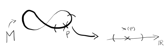
Consider $M \subseteq \mathbb{R}^2$ defined by the following picture:
$(M,\mathcal{O}_{\mathrm{standard}|M})$ is a 1-dimensional topological manifold: around any point $p \in M$, we can map a ball $B_r(p)$ around $p$ continuously (with continuous inverse) to $\mathbb{R}$.
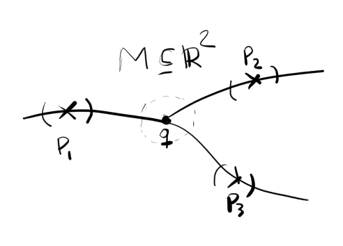
Consider the following $M \subseteq \mathbb{R}$:
$(M, \mathcal{O}_{\mathrm{standard}|M})$ is a topological space, but not a topological manifold: although you can chart the regions around $p_1,p_2$ and $p_3$ in $\mathbb{R}$, you can't chart any region around $q$ in either $\mathbb{R}$ (can't map continuously from region around bifurcation point to an interval) or $\mathbb{R}^2$ (the preimage of a 2-dimensional ball would necessarily include points outside of $M$).
Some terminology:
as stated above, $(\mathcal{U}, x)$ is a chart of $(M, \mathcal{O})$.
$\mathcal{A} = \{(\mathcal{U}_\alpha, x_\alpha) \mid \alpha \in A\}$ is an atlas if $M = \bigcup_\alpha \mathcal{U}_\alpha$.
$x \colon \mathcal{U} \to x(\mathcal{U}) \subseteq \mathbb{R}^d$ is a chart map.
we can write $x(p) = (x^1(p), \dots, x^d(p))$ where $x^i \colon \mathcal{U} \to \mathbb{R}$ for $i=1,\dots,d$ is called a coordinate map.
Choosing different charts roughly amounts to choosing different coordinates.
Chart transition maps
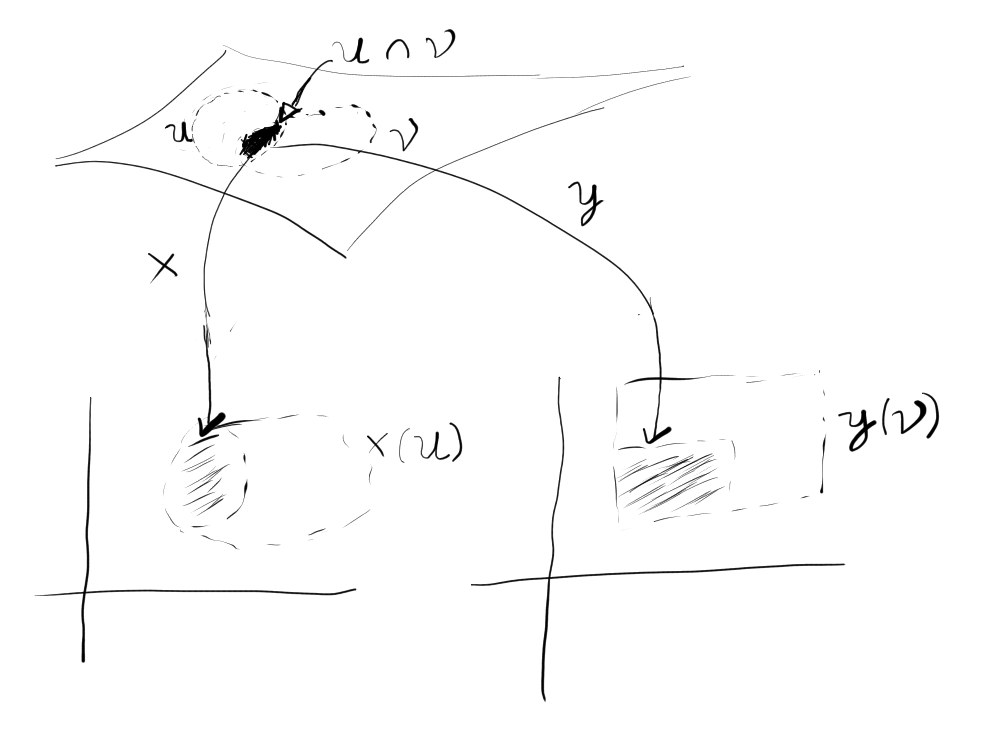
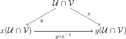
Consider two charts $(\mathcal{U}, x), (\mathcal{V}, y)$ with overlapping regions, i.e. $\mathcal{U} \cap \mathcal{V} \neq \emptyset$.
The chart transition map is given by $y \circ x^{-1}$.
This map tells you how to glue together different charts of an atlas.
Manifold philosophy
Often it's necessary to define properties (like continuity) of real-world objects (say a curve $\gamma \colon \mathbb{R} \to M$) on a chart representative (i.e. $x \circ \gamma$) of the object. This allows "lifting" the concepts we know from $\mathbb{R}$ to manifolds.
The disadvantage of this approach is that the property might be ill-defined. It might turn out that the property is specific to the choice of chart.
Let $\gamma \colon \mathbb{R} \to \mathcal{U} \subset M$. If we show that the property holds for a specific chart $x$ and later show that it'd also hold if we transitioned to a different (arbitrary) chart $y$, then we say that the property holds for $\gamma$.
Consider continuity. Let's say we show that $x \circ \gamma$ is continuous. Is $y \circ \gamma$ continuous? We have
By assumption, $x \circ \gamma$ is continuous and both $y$ and $x^{-1}$ are continuous, hence $y \circ x^{-1}$ is continuous, hence $y \circ \gamma$ is continuous.
However: say $x \circ \gamma \colon \mathbb{R} \to \mathbb{R}^d$ is differentiable. Can we say $y \circ \gamma$ is differentiable? In general we cannot, because the chart transition map $y \circ x^{-1}$ might not be differentiable. In order to talk about differentiability, we need to place restrictions on the type of chart we're allowed to consider.
Multilinear algebra
Spacetime is not equipped with a vector space structure; the notion of adding and scaling points in spacetime is not well-defined.
However, we are also interested in tangent spaces, which are vector spaces.
So, it's time for a detour. In order to understand tangent spaces $T_p M$ we need to understand $C^{\infty}(M)$. We'll also look at the notion of tensors, which are more easily understood abstractly.
An $\mathbb{R}$-vector space $(V, +, \cdot)$ is a set $V$ equipped with $+ \colon V \times V \to V$ and $\cdot \colon \mathbb{R} \times V \to V$ satisfying the following properties:
$u,v \in V \implies u + v = v + u$
$u,v,w \in V \implies (u + v) + w = u + (v + w)$
There exists an element $\mathbf{0} \in V$ with $u + \mathbf{0} = \mathbf{0} + u = u$.
For any $u \in V$, there exists $v \in V$ with $u + v = \mathbf{0}$. (We call $v := -u$.)
$\lambda \in \mathbb{R}, u,v \in V \implies \lambda \cdot (u + v) = \lambda \cdot u + \lambda \cdot v$.
$\lambda,\mu \in \mathbb{R}, u \in V \implies (\lambda + \mu) \cdot u = \lambda \cdot u + \mu \cdot u$.
$1 \cdot u = u$.
Let $P := \{p \colon (-1,+1) \to \mathbb{R} \mid \sum_{n=0}^N p_n x^n\}$ be the set of polynomials of degree $N$ equipped with $+ \colon P \times P \to P$ and $\cdot \colon \mathbb{R} \times P \to P$ defined by $(p + q)(x) := p(x) +_\mathbb{R} q(x)$ and $(\lambda \cdot p)(x) := \lambda \cdot_\mathbb{R} p(x)$. Then $(P,+,\cdot)$ is an $\mathbb{R}$-vector space.
Generally it's not very meaningful to talk about vectors individually. It's the structure of the vector space that matters.
Linear maps
These are maps that preserve the vector space structure.
Definition. Let $(V,+_V,\cdot_V),(W,+_W,\cdot_W)$ be vector spaces. Then $\varphi \colon V \to W$ is called linear if for $\lambda \in \mathbb{R}, u,v \in V$, the following properties are satisfied:
Example. Consider the following map over the vector space $P$ of polynomials of fixed degree $N$:
$$\begin{align*}
\delta \colon P &\to P \\
p &\mapsto \delta(p) := p'
\end{align*}$$
Where $p'$ is the derivative of $p$. $\delta$ is a linear map, known as the differentiation operator.
Notation. If $\varphi \colon V \to W$ is linear we often write $\varphi \colon V \xrightarrow{\sim} W$.
Vector space of homomorphisms
Definition. Let $(V,+,\cdot),(W,+,\cdot)$ be vector spaces. The set
$$\mathrm{Hom}(V, W) := \{\varphi \colon V \xrightarrow{\sim} W\}$$
can be made into a vector space (with pairwise addition and multiplication by scalar). It's the vector space of homomorphisms from $V$ to $W$.
Dual vector space
Definition. Let $(V,+,\cdot)$ be a vector space. The vector space $V^* := \mathrm{Hom}(V, \mathbb{R})$ is called the dual vector space (to $V$).
Informally, we call an element $\varphi \in V^*$ a covector.
Example. Let
$$\begin{align*}
I \colon P &\xrightarrow{\sim} \mathbb{R} \\
p &\mapsto \int_0^1 p(x)\,\mathrm{d}x
\end{align*}$$
$I$ is a linear map and hence a covector, called the integration operator.
Tensors
Definition. Let $(V,+,\cdot)$ be a vector space. An $(r,s)$-tensor $T$ over $V$ is a map
$$T \colon \underbrace{V^* \times \dots \times V^*}_r \times \underbrace{V \times \dots \times V}_s \to \mathbb{R}$$
which is multilinear; i.e. it's linear on each of its $r+s$ inputs.
Given $T \colon V^* \times V \xrightarrow{\sim} \mathbb{R}$, it's easy to construct (using the fact that for finite-dimensional vector spaces, $(V^*)^* \cong V$) a function $\varphi_T \colon V \xrightarrow{\sim} V$. Conversely, given $\varphi \colon V \xrightarrow{\sim} V$, it's easy to construct $T_\varphi \colon V^* \times V \xrightarrow{\sim} \mathbb{R}$. More generally, the two views of tensors as multilinear maps $V^r \to V^s$ and of tensors as multilinear maps $(V^*)^r \times V^s \to \mathbb{R}$ are equivalent.
Vectors and covectors as tensors
If $\varphi \in V^*$, then $\varphi$ is a $(0,1)$-tensor by definition. Similarly, if $v \in V \cong (V^*)^*$, then we can write $v \colon V^* \xrightarrow{\sim} \mathbb{R}$, hence $v$ is a $(1,0)$-tensor. Also, linear maps over $V$ are $(1,1)$-tensors.
Basis for a vector space
Let $(V,+,\cdot)$ be a vector space. A subset $B \subset V$ is a (Hamel) basis of $V$ if for every $v \in V$, there's a unique set $\{f_1,\dots,f_n\} \subset B$ and unique $v^1,\dots,v^n \in \mathbb{R}$ with $v = v^1 f_1 + \dots + v^n f_n$.
If $B$ has finitely many elements, say $d$, we call $\mathrm{dim}\,V := d$, the dimension of $V$.
Any two bases of $V$ have the same dimension.
Having chosen a basis $e_1,\dots,e_n$ of a vector space $(V,+,\cdot)$, we may uniquely associate $v \mapsto (v^1,\dots,v^n)$ for any element $v \in V$, where $v = v^1 e_1 + \dots + v^n e_n$. These are called the components of $v$ with respect to the basis $e_1,\dots,e_n$.
Basis for dual space
Choose a basis $e_1,\dots,e_n$ for $V$ and a basis $\epsilon^1,\dots,\epsilon^n$ for $V^*$. It's useful to require that, once $e_1,\dots,e_n$ are chosen, we have $\epsilon^a e_b = \delta_{ab}$, where $\delta_{ij} = 1$ if $i = j$ and $\delta_{ij} = 0$ if $i \neq j$. If the basis $\epsilon^1,\dots,\epsilon^n$ satisfies this, we call it the dual basis of $V^*$.
Let $P$ be the vector space of polynomials of degree at most 3. The polynomials $e_0(x) = 1, e_1(x) = x, e_2(x) = x^2, e_3(x) = x^3$ form a basis of $P$. The set $\{\epsilon^a\}_{0 \leq a \leq 3}$ defined by
$$\epsilon^a(p(x)) := \frac{1}{a!} \left(\frac{dp}{dx}\right)_{x=0}$$
can be shown to satisfy $\epsilon^a(e_b(x)) = \delta_{ab}$, so it is the dual basis of $P$.
Components of tensors
Let $T$ be an $(r,s)$-tensor over a finite-dimensional vector space $V$. Define the $(r+s)^{\mathrm{dim}\,V}$ real numbers
$$T^{i_1,\dots,i_r}_{j_1,\dots,j_s} := T(\epsilon^{i_1},\dots,\epsilon^{i_r},e_{j_1},\dots,e_{j_s})$$
where the indices go from 1 to $\mathrm{dim}\,V$.
These are the components of the tensor with respect to the chosen basis (and its corresponding dual basis).
Einstein summation convention
Whenever an index appears twice in a single term, there's an implicit summation over all the values of the term.
Typically, we write basis elements (vectors) with subscripts and vector components with superscripts. Conversely, we write dual basis elements (covectors) with superscript and covector components with subscripts.
Let $T$ be a $(1,1)$-tensor and $T^i_j := T(\epsilon^i,e_j)$. For an arbitrary covector $\varphi$ and vector $v$, we can write
(note the use of the Einstein summation convention.)
Differentiable manifolds
From the definition of topological manifold, it is not possible to talk about differentiability.
We want to define a notion of differentiable curves ($\mathbb{R} \to M$), functions ($M \to \mathbb{R}$), and maps ($M \to N$).
A possible strategy is to choose a chart $(\mathcal{U},x)$, restrict the curve to the portion that lies within the chart domain $\mathcal{U}$, and look at the map $x \circ \gamma \colon \mathbb{R} \to x(\mathcal{U}) \subseteq \mathbb{R}$.
We can apply the calculus notion of differentiability to this induced curve and try to "lift" it to a notion of differentiability of the curve $\gamma$ on the manifold.
Problem: can this be well-defined? Does this notion depend on the choice of chart?
Consider two charts, $(\mathcal{U},x), (\mathcal{V},y)$ and the restriction $\gamma \colon \mathbb{R} \to \mathcal{U} \cap \mathcal{V}$. We have two induced curves $x \circ \gamma$ and $y \circ \gamma$. If $x \circ \gamma$ is differentiable, what can we say about $y \circ \gamma$? We have
$$y \circ \gamma = (y \circ x^{-1}) \circ (x \circ \gamma)$$
We only know that the transition map $y \circ x^{-1}$ is continuous, and generally, the composition of a continuous function and a differentiable function is not differentiable.
Compatible charts
So far we've only taken charts of the maximal atlas $\mathcal{A}$ of $(M,\mathcal{O})$. Can we choose a more restricted atlas such that transition maps are always differentiable?
Two charts $(\mathcal{U},x),(\mathcal{V},y)$ are called compatible with respect to a property $p$ if either $\mathcal{U} \cap \mathcal{V} = \emptyset$ or the maps
$$\begin{align*}
y \circ x^{-1}\,&\colon\,x(\mathcal{U} \cap \mathcal{V}) \to y(\mathcal{U} \cap \mathcal{V}) \\
x \circ y^{-1}\,&\colon\,y(\mathcal{U} \cap \mathcal{V}) \to x(\mathcal{U} \cap \mathcal{V})
\end{align*}$$
have the property $p$ (as maps $\mathbb{R}^d \to \mathbb{R}^d$).
An atlas is called a $p$-compatible atlas (or simply $p$-atlas) if any two charts in it are $p$-compatible.
For example, in a $C^k$-atlas every two charts are $C^k(\mathbb{R} \to \mathbb{R})$-compatible. Note that every atlas is a $C^0$-atlas since transition maps are always continuous.
Any $C^k$-atlas of a topological manifold with $k \geq 1$ contains a $C^{\infty}$-atlas (also named a smooth atlas).
So we may consider without loss of generality smooth manifolds (that is, manifolds equipped with a smooth atlas), unless we need to defined Taylor expandability (needs real analytic atlas) or complex differentiability (needs complex analytic atlas).
Diffeomorphisms
Consider two sets $M,N$. If there's no specified structure in $M$ or $N$, the only structure-preserving maps we can talk about are bijective maps.
Now consider two manifolds, $(M,\mathcal{O}_M),(N,\mathcal{O}_N)$. We say that they are homeomorphic if there's a bijection $\varphi \colon M \to N$ with both $\varphi,\varphi^{-1}$ continuous.
Now consider two smooth manifolds, $(M,\mathcal{O}_M,\mathcal{A}_M),(N,\mathcal{O}_N,\mathcal{A}_N)$. We say that they are diffeomorphic if there's a bijection $\varphi \colon M \to N$ where $\varphi,\varphi^{-1}$ are $C^\infty$ maps. Note that for this notion to make sense we need to choose charts in $M$ and $N$: if we take $(\mathcal{U},x) \in \mathcal{A}_M$ and $(\mathcal{V},y) \in \mathcal{A}_N$, then we say that $\varphi$ is $C^\infty$ if $y \circ \varphi \circ x^{-1} \colon x(\mathcal{U}) \to y(\mathcal{V})$ is $C^\infty$.
The number of $C^\infty$-manifolds one can make out of a given $C^0$-manifold is, up to diffeomorphism,
Consider a curve $\gamma$ on a manifold $M$. What is the velocity of $\gamma$ at a point $p$?
Velocities
Let $(M,\mathcal{O},\mathcal{A})$ be a smooth manifold and $\gamma \colon \mathbb{R} \to M$ be a curve which is at least $C^1$ (i.e. pick a chart $(\mathcal{U},x)$, then $x \circ \gamma$ is differentiable and the derivative is continuous) and let $p = \gamma(\lambda_0)$ for some $\lambda_0 \in \mathbb{R}$. The velocity of $\gamma$ at $p$ is the linear map
For each $p \in M$, the tangent space to $M$ at $p$ is defined as
$$T_p M := \{v_{\gamma,p} \mid \gamma\,\,\textrm{is a smooth curve that passes through}\,\,p\}$$
It's useful to picture the tangent space as a plane that touches the manifold at $p$ and is tangent to it. However, note that the definition makes no reference to an ambient space: it's defined in the manifold itself. That is, it only uses intrinsic properties of the manifold.
$T_p M$ can be made into a vector space. (Define two operations $+ \colon T_p M \times T_p M \to \mathrm{Hom}(C^\infty(M), \mathbb{R})$, $\cdot \colon \mathbb{R} \times T_p M \to \mathrm{Hom}(C^\infty(M), \mathbb{R})$ and construct a curve whose velocity at $p$ equals that of the resulting functions.)
This implies that although the sum of two curves generally depends on the choice of chart, their velocities at a specific point can be added in a chart-independent manner.
Components of a vector with respect to a chart
Let $(\mathcal{U},x)$ be a chart in a smooth atlas. Let $\gamma \colon \mathbb{R} \to \mathcal{U}$ with $\gamma(0) = p$. We have
where $\partial_i$ denotes the partial derivative in the $i$th direction. We write
$$\begin{align*}
\left(\frac{\partial f}{\partial x^i}\right) &:= \partial_i (f \circ x^{-1}) (x(p)) \\
\dot{\gamma}_x^i(0) &:= (x^i \circ \gamma)'(0).
\end{align*}$$
With this notation, we have $v_{\gamma,p} = \dot{\gamma}_x^i(0) \left(\dfrac{\partial}{\partial x^i}\right)_p$.
$\dot{\gamma}_x^i(0)$ are the components of the velocity with respect to the chart $x$.
The elements $\left(\dfrac{\partial}{\partial x^i}\right)_p$ can be shown to be a basis of $T_p \mathcal{U}$, sometimes called the chart-induced or coordinate-induced basis of $T_p M$.
Change of vector components under change of chart
First, some terminology. We often write something $X \in T_p M$, which means that there's some curve $\gamma$ through $p$ with $X = v_{\gamma,p}$. We can write $X = X^i \left(\dfrac{\partial}{\partial x^i}\right)_p$ where $X^i,\dots,X^d \in \mathbb{R}$.
Let $(\mathcal{U},x),(\mathcal{V},y)$ be overlapping charts and $p \in \mathcal{U} \cap \mathcal{V}$ and let $X \in T_p M$. We can write $X$ in two ways:
Let's consider the dual space $(T_p M)^* = \{ \varphi\,\colon T_p M \xrightarrow{\sim} \mathbb{R} \}$. Consider the function $(\mathrm{d}f)_p \in (T_p M)^*$ defined by $(\mathrm{d}f)_p(X) := X f$ (where $X \in T_p M$). $(\mathrm{d}f)_p$ is called the gradient of $f$ at $p$. The components of the gradient are given by
Consider a chart $(\mathcal{U},x)$ and let $x^i\,\colon \to \mathbb{R}$ be the components of $x$. The set $(\mathrm{d}x^1)_p,\dots,(\mathrm{d}x^d)_p$ is the dual basis of $T_p^* M$.
Change of components of covector under change of chart
Let $\omega = T_p^* M$. We can write $\omega = \omega_{(x),i} (\mathrm{d}x^i)_p = \omega_{(y),j} (\mathrm{d}y^j)_p$. Similar to the calculation for vectors, we can show that
$$E \xrightarrow{\pi} M$$
where $E$ is a smooth manifold (the total space), $\pi$ is a smooth surjective map (the projection map) and $M$ is a smooth manifold (the base space).
(Mental picture: take $E$ to be a cylinder and $M$ to be a circle.)
Take a bundle $E \xrightarrow{\pi} M$ and $p \in M$. The fiber on $p$ is the preimage $\pi^{-1}(\{p\}) \subseteq E$. A section of a bundle is a function $\sigma\,\colon M \to E$ with $\pi \circ \sigma = \mathrm{id}_M$.
(Aside: in quantum mechanics, "wave functions" $\psi\,\colon M \to \mathbb{C}$ are actually $\mathbb{C}$-sections of $M$.)
Tangent bundle of a smooth manifold
Let $(M,\mathcal{O},\mathcal{A})$ be a smooth manifold. We'd like to construct a tangent bundle $TM \xrightarrow{\pi} M$. Let
$$TM := \bigsqcup_{p \in M} T_p M$$
where $\sqcup$ denotes the disjoint union. We define $\pi\,\colon TM \to M$ as follows: if $X \in T_p M$, then $\pi(X) = p$. This is well-defined because the union is disjoint: given $X \in TM$, we know which $T_p M$ includes $X$. $\pi$ is also surjective because the union is taken over all $p \in M$.
To make $TM$ into a smooth manifold, we need to define a topology on it. We'll take the coarsest topology (i.e., topology with the least number of elements) on $TM$ such that $\pi$ is continuous. It is defined as
$$\mathcal{O}_{TM} := \{ \pi^{-1}(\mathcal{U}) \mid \mathcal{U} \in \mathcal{O} \}.$$
By definition $\pi$ takes sets in $\mathcal{O}_{TM}$ to sets in $\mathcal{O}$, hence it is continuous.
Now we need a smooth atlas. We'll build it using the atlas $\mathcal{A}$ for the base space. Any given $X \in TM$ has a base point $p \in M$ and is a vector $T_p M$, hence to describe it we can take a chart $(\mathcal{U}, x)$ in $\mathcal{A}$ and use it to write down the components of $p$ with respect to it and the vector components of $X$ with respect to the induced chart in $T_p M$.
The coordinates of $p$ with respect to $(\mathcal{U}, x)$ are $(x^i \circ \pi)(X)$, and the vector components of $X$ are given by $(\mathrm{d}x^i)_{\pi(X)}(X)$. Hence we can construct $\mathcal{A}_{TM}$ as
$$\mathcal{A}_{TM} := \{ (T\mathcal{U}, \xi_x) \mid (\mathcal{U},x) \in \mathcal{A} \}$$
where $\xi_x$ is given by
$$\begin{align*}
\xi_x\,&\colon T\mathcal{U} \to \mathbb{R}^{2 \cdot \mathrm{dim} M} \\
X &\mapsto ((x^1 \circ \pi)(X), \dots, (x^d \circ \pi)(X), (\mathrm{d}x^1)_{\pi(X)}(X),\dots,(\mathrm{d}x^d)_{\pi(X)}(X))
\end{align*}$$
This can be shown to be a smooth atlas.
Vector fields
A smooth vector field is a smooth map $\chi \colon M \to TM$ which is a section of $TM$ (i.e., $\pi \circ \chi = \mathrm{id}_M$).
The $C^\infty(M)$-module $\Gamma(TM)$.
Let $\Gamma(TM)$ be the collection of all vector fields on $M$ and define
$$\begin{align*}
\chi f\,&\colon M \to \mathbb{R} \\
&p \mapsto \chi(p) f
\end{align*}$$
So we can define operations $+\,\colon \Gamma(TM) \times \Gamma(TM) \to \Gamma(TM)$ and $\cdot\,\colon C^\infty(M) \times \Gamma(TM) \to \Gamma(TM)$ by $(\chi + \tilde{\chi}) f := (\chi f) + (\tilde{\chi} f), f \cdot (\chi g) := \chi (f g)$.
However, $C^\infty(M)$ is a ring (and not a field), hence $\Gamma(TM)$ is not a vector space, but a module. This means that we can't always pick a basis for $\Gamma(TM)$. Simple counterexample: there's no smooth nonvanishing vector field on a sphere (hairy ball theorem).
Note that chart-induced tangent vector fields $\dfrac{\partial}{\partial x^i}$ define a basis in the chart's domain, which does not contradict the statement above. We can expand a vector field $\chi$ on the domain of a chart $(U, x)$ as follows. For a given $p \in U$, $\chi(p) \in T_p U$, so we can write $\chi(p) = \chi_{(x)}^i(p) \left(\dfrac{\partial}{\partial x^i} \right)_p$. We can define $\chi_{(x)}^i \colon U \to \mathbb{R}$, $\dfrac{\partial}{\partial x^i} \colon U \to \mathbb{R}$; these can be shown to be smooth functions. This gives a decomposition $\chi = \chi_{(x)}^i \dfrac{\partial}{\partial x^i}$, where here addition and multiplication are taking place in $\Gamma(TU)$.
Tensor fields
Like $\Gamma(TM)$, we can consider the module of covector fields $\Gamma(T^* M)$, by defining the cotangent bundle just as we did above for the tangent bundle, but starting from the cotangent space $T_p^* M = \{\varphi \colon T_p M \xrightarrow{\sim} \mathbb{R}\}$.
An $(r,s)$-tensor field $T$ is a $C^\infty(M)$-multilinear map
$$T\,\colon \underbrace{\Gamma(T^* M) \times \cdots \times \Gamma(T^* M)}_r \times \underbrace{\Gamma(TM) \times \cdots \Gamma(TM)}_s \xrightarrow{\sim} C^\infty(M)$$
(Note that $\mathbb{R}$-multilinearity is not enough to defined a tensor field.)
where $(\chi f)(p) := \chi(p) f$. $\mathrm{d} f$ is a $(0,1)$-tensor field.
Connections
So far: a vector field $X$ provides a directional derivative $\nabla_X f := X f$ of a function $f \in C^\infty(M)$.
We currently have the following objects:
$$\begin{align*}
X\,\colon C^\infty(M) &\to C^\infty(M) \\
\mathrm{d}f\,\colon \Gamma(TM) &\to C^\infty(M) \\
\nabla_X \,\colon C^\infty(M) &\to C^\infty(M)
\end{align*}$$
which act the same way ($Xf = (\mathrm{d} f)(X) = \nabla_X f$). However, as we'll see, we can generalize $\nabla_X$ to take a $(p,q)$-tensor field into a $(p,q)$-tensor field. For this we'll need to add new structure to the manifold, hence the new notation.
Directional derivatives of tensor fields
What properties should $\nabla_X$ acting on a tensor field have?
A (linear) connection (or covariant derivative) on a smooth manifold $(M, \mathcal{O}, \mathcal{A})$ is a map taking a pair $(X,T)$ where $X$ is a vector (field) and $T$ is a $(p,q)$-tensor field and sends them to a $(p,q)$-tensor (field) $\nabla_X T$, satisfying
(extension) $\nabla_X f = X f$ for every $f \in C^\infty(M)$ (i.e., a $(0,0)$-tensor field).
(additivity) $\nabla_X (T + S) = \nabla_X T + \nabla_X S$ for tensor fields $T,S$.
(Leibniz rule) $\nabla_X T(\omega, Y) = (\nabla_X T)(\omega, Y) + T(\nabla_X \omega, Y) +T(\omega, \nabla_X Y)$ if $T$ is a $(1,1)$-tensor (and analogously for general $(p,q)$-tensors).
$\nabla_{f X + Z} T = \nabla_{f X} T + \nabla_Z T = f \cdot \nabla_X T + \nabla_Z T$ for vector fields $X,Z$ and $f \in C^\infty(M)$.
A manifold with connection is a quadruple $(M,\mathcal{O},\mathcal{A},\nabla)$.
$\nabla_X$ is an extension of $X$ to act on arbitrary tensor fields. We can think of $\nabla$ as an extension of $\mathrm{d}$ (as in $\mathrm{d} f$).
If we want to define a connection, how much freedom do we have in choosing $(M,\mathcal{O},\mathcal{A})$?
Consider $\nabla_X Y$ where $X,Y$ are vector fields and choose a chart $(\mathcal{U},x)$. We have
$$\begin{align*}
\nabla_X Y &= \nabla_{X^i \frac{\partial}{\partial x^i}} \left(Y^j \frac{\partial}{\partial x^j}\right) \\
&= X^i \left(\nabla_{\frac{\partial}{\partial x^i}} Y^j\right) \frac{\partial}{\partial x^j} + X^i Y^j \nabla_{\frac{\partial}{\partial x^i}} \frac{\partial}{\partial x^j} \\
&= X^i \left(\frac{\partial Y^j}{\partial x^i}\right) \frac{\partial}{\partial x^j} + X^i Y^j \Gamma_{ji}^q \frac{\partial}{\partial x^q}
\end{align*}$$
for some $\Gamma_{ji}^q$. These are the connection coefficients, which are functions on $M$. These are obtained by expanding $\nabla_{\frac{\partial}{\partial x^i}} \frac{\partial}{\partial x^j}$ (which is a vector field on $\mathcal{U}$) with respect to the chart $(\mathcal{U},x)$. More precisely, they are the $(\mathrm{dim}\,M)^3$ functions
This means that on a chart domain $\mathcal{U}$, the choice of the functions $\Gamma_{jk}^i$ suffices to fix the action of $\nabla$ on a vector field. It can be shown that the same functions also fix the action on any tensor field.
The key observation for this is to note that the expansion for $\nabla_{\frac{\partial}{\partial x^j}} (\mathrm{d} x^i)$ can be written using the same coefficients. We have
$$
\nabla_{\frac{\partial}{\partial x^j}} \left(\mathrm{d} x^i \left(\frac{\partial}{\partial x^k}\right) \right) = \frac{\partial}{\partial x^j} (\delta_k^i) = 0.
$$
But on the other hand, by the Leibniz rule we have
$$\begin{align*}
\nabla_{\frac{\partial}{\partial x^j}} \left(\mathrm{d} x^i \left(\frac{\partial}{\partial x^k}\right) \right) &= \left( \nabla_{\frac{\partial}{\partial x^j}} \mathrm{d}x^i \right) \left(\frac{\partial}{\partial x^k} \right) + \mathrm{d} x^i \left(\nabla_{\frac{\partial}{\partial x^j}} \frac{\partial}{\partial x^k}\right) \\
&= \nabla_{\frac{\partial}{\partial x^j}} (\mathrm{d}x^i) \left(\frac{\partial}{\partial x^k} \right) + \mathrm{d} x^i \Gamma_{kj}^q \frac{\partial}{\partial x^q} \\
&= \nabla_{\frac{\partial}{\partial x^j}} (\mathrm{d}x^i) \left(\frac{\partial}{\partial x^k} \right) + \Gamma_{kj}^i \frac{\partial}{\partial x^i}.
\end{align*}$$
Given a point $p \in M$, it is possible to construct a chart $(\mathcal{U},x)$ with $p \in \mathcal{U}$ such that $\Gamma_{(x),jk}^i(p) = 0$. This is called a normal coordinate chart of $\nabla$ at $p \in M$.
Note, however, that this won't necessarily be the case in any neighborhood of $p$. As we'll see, that when the coefficients are null everywhere, we are in a so-called flat manifold.